Soft body dynamics is about simulating realistic deformable objects. We’ll use it here to simulate a curtain and a set of ragdolls that you can interact with and fling around the screen. It’ll be fast, stable, and simple enough to do with high school level mathematics.
Note: Although this tutorial is written in Processing and compiled with Java, you should be able to use the same techniques and concepts in almost any game development environment.
Final Result Preview
In this demo, you can see a big curtain (showing off the fabric simulation), and a number of little stickmen (showing off the ragdoll simulation):
You can try the demo yourself, too. Click and drag to interact, press ‘R’ to reset, and hit ‘G’ to toggle the gravity.
Step 1: A Point and Its Motion
The building blocks of our game with be the Point. For the sake of avoiding ambiguity, we’ll call it the PointMass. The details are in the name: it’s a point in space, and it represents an amount of mass.
The most basic way to implement physics for this point is to “forward” its velocity in some way.
x = x + velX
y = y + velY
Step 2: Timesteps
We can’t assume our game will run at the same speed all the time. It might run at 15 frames per second for some users, but at 60 for others. It’s best to account for frame rates of all ranges, which can be done using a timestep.
x = x + velX * timeElapsed
y = y + velY * timeElapsed
This way, if a frame were to take longer to elapse for one person than for another, the game would still run at the same speed. For a physics engine, however, this is incredibly unstable.
Imagine if your game freezes for a second or two. The engine would over-compensate for that, and move the PointMass past several walls and objects that it would otherwise have detected a collision with. Thus, not only would collision detection be affected, but also the method of constraint solving we’ll be using.
How can we have the stability of the first equation, x = x + velX, with the consistency of the second equation, x = x + velX * timeElapsed? What if, maybe, we could combine the two?
That is exactly what we’ll do. Imagine if our timeElapsed was 5. We could do the exact same thing as the latter equation, but with a higher accuracy and resolution, by calling x = x + velX 5 times.
elapsedTime = lastTime - currentTime
lastTime = currentTime // reset lastTime

// add time that couldn't be used last frame
elapsedTime += leftOverTime

// divide it up in chunks of 16 ms
timesteps = floor(elapsedTime / 16)

// store time we couldn't use for the next frame.
leftOverTime = elapsedTime - timesteps

for (i = 0; i < timesteps; i++) {
     x = x + velX * 16
     y = y + velY * 16

     // solve constraints, look for collisions, etc.
}
The algorithm here uses a fixed timestep larger than one. It finds the elapsed time, breaks it up into fixed sized “chunks”, and pushes the remaining amount of time over to the next frame. We run the simulation little by little for every chunk our elapsed time is broken up into.
I picked 16 for the timestep size, to simulate the physics as if it were running at approximately 60 frames per second. Conversion from elapsedTime to frames per second can be done with some math: 1 second / elapsedTimeInSeconds.
1s / (16ms/1000s) = 62.5fps, so a 16ms timestep is equivalent to 62.5 frames per second.
Step 3: Constraints
Constraints are restrictions and rules added to the simulation, guiding where PointMasses can and cannot go.
They can be simple as this boundary constraint, for preventing PointMasses moving off the left edge of the screen:
if (x < 0) {
     x = 0
     if (velX < 0) {
          velX = velX * -1
     }
}
Adding the constraint for the right edge of the screen is done similarly:
if (x > width) {
     x = width
     if (velX > 0) {
          velX = velX * -1
     }
}
Doing this for the y axis is a matter of changing every x to a y.
Having the right kind of constraints can result in very beautiful and captivating interactions. Constraints can also become extremely complex. Try imagining simulating a vibrating basket of grains with none of the grains intersecting, or a 100-joint robotic arm, or even something simple as a stack of boxes. The typical process involves finding points of collisions, finding the exact time of collision, and then finding the right force or impulse to apply to each body to prevent that collision.
Comprehending the amount of complexity a set of constraints can have can be difficult, and then solving those constraints, in real time is even more difficult. What we’ll be doing is simplifying constraint solving significantly.
Step 4: Verlet Integration
A mathematician and programmer named Thomas Jakobsen explored some ways of simulating the physics of characters for games. He proposed that accuracy is not nearly as important as believability and performance. The heart of his whole algorithm was a method used since the 60s to model molecular dynamics, called Verlet Integration. You might be familiar with the game Hitman: Codename 47. It was one of the first games to use ragdoll physics, and uses the algorithms Jakobsen developed.
Verlet Integration is the method we’ll use to forward the position of our PointMass. What we did prior, x = x + velX, is a method called Euler Integration (which I also used in Coding Destructible Pixel Terrain).
The major difference between Euler and Verlet Integration is how velocity is implemented. Using Euler, a velocity is stored with the object and is added on to the object’s position every frame. Using Verlet, however, applies inertia by using the previous and current position. Take the difference in the two positions, and add it to the latest position to apply inertia.
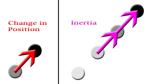
// Inertia: objects in motion stay in motion.
velX = x - lastX
velY = y - lastY

nextX = x + velX + 0.5 * accX * timestepSq
nextY = y + velY + 0.5 * accY * timestepSq

lastX = x
lastY = y

x = nextX
y = nextY
We added acceleration in there for gravity. Other than that, accX and accY won’t be necessary for solving for collisions. Using Verlet Integration, we no longer need to do any sort of impulse or force solving for collisions. Changing the position alone will be enough to have a stable, realistic, and fast simulation. What Jakobsen developed is a linear substitute for something that’s otherwise nonlinear.
Step 5: Link Constraints
The benefits of Verlet Integration can be best shown through example. In a fabric engine, we’ll not only have PointMasses, but also links in between them. Our “links” will be a distance constraint between two PointMasses. Ideally, we want two PointMasses with this constraint to always be at a certain distance apart.
Whenever we solve this constraint, Verlet Integration should keep these pointmasses in motion. For example, if one end were to be moved quickly down, the other end should follow it like a whip through inertia.
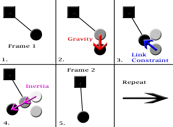
We’ll only need one link for each pair of PointMasses attached to each other. All the data you’ll need in the link is the PointMasses and the resting distances. Optionally you can have stiffness, for more of a Spring constraint. In our demo we also have a “tear sensitivity,” which is the distance at which the link will get removed.
I’ll only explain restingDistance here, but the tear distance and stiffness are both implemented in the demo and the source code.
Link {
     restingDistance
     tearDistance
     stiffness

     PointMass A
     PointMass B
     solve() {
          math for solving distance
     }
}
You can use linear algebra to solve for the constraint. Find the distances between the two, determine how far along the restingDistance they are, then translate them based on that and their differences.
// calculate the distance
diffX = p1.x - p2.x
diffY = p1.y - p2.y
d = sqrt(diffX * diffX + diffY * diffY)

// difference scalar
difference = (restingDistance - d) / d

// translation for each PointMass. They'll be pushed 1/2 the required distance to match their resting distances.
translateX = diffX * 0.5 * difference
translateY = diffY * 0.5 * difference

p1.x += translateX
p1.y += translateY

p2.x -= translateX
p2.y -= translateY
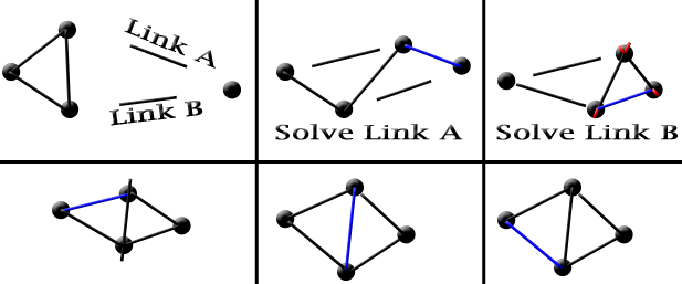
In the demo, we account for mass and stiffness as well. There are some problems in solving this constraint. When there are more than two or three PointMasses linked to each other, solving some of these constraints may violate other constraints previously solved.

Thomas Jakobsen encountered this problem as well. At first, one might create a system of equations, and solve for all of the constraints at once. This would increase in complexity rapidly though, and would be difficult to add more than even just a few links into the system.
Jakobsen developed a method that might seem silly and naive at first. He created a method called “relaxation,” where instead of solving for the constraint once, we solve for it several times. Each time we reiterate and solve for the links, the set of links become closer and closer to all being solved.
Step 6: Bring It Together
To recap, here is how our engine works in pseudocode. For a more specific example, check out the demo’s source code.
animationLoop {
     numPhysicsUpdates = however many we can fit in the elapsed time
     for (each numPhysicsUpdates) {
          // (with constraintSolve being any number 1 or higher. I typically use 3
          for (each constraintSolve) {
               for (each Link constraint) {
                    solve constraint
               } // end link constraint solves
          } // end constraints

          update physics // (use verlet!)
     } // end physics update

     draw points and links
}
Step 7: Add a Fabric
Now we can construct the fabric itself. Creating the links should be fairly simple: link to the left when the PointMass isn’t the first one on its row, and link up when it isn’t the first in its column.
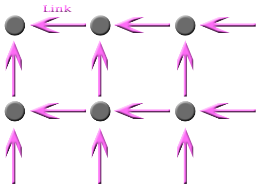
The demo uses a one-dimensional list to store PointMasses, and finds points to link to using x + y * width.
// we want the y loop to be on the outside, so it scans row-by-row instead of column-by-column
for (each y from 0 to height) {
     for (each x from 0 to width) {
          new PointMass at x,y

          // attach to the left
          if (x != 0)
               attach PM to last PM in list

          // attach to the right
          if (y != 0)
               attach PM to PM @ ((y - 1) * (width+1) + x) in list

          if (y == 0)
                pin PM

          add PM to list
     }
}
You might notice in the code that we also have “pin PM.” If we don’t want our curtain to fall, we can lock the top row of PointMasses to their starting positions. To program a pin constraint, add some variables to keep track of the pin location, and then move the PointMass to that position after every constraint solve.
Step 8: Add Some Ragdolls
Ragdolls were Jakobsen’s original intentions behind his use of Verlet Integration. First we’ll start with the heads. We’ll create a Circle constraint which will only interact with the boundary.
Circle {
     PointMass
     radius
     solve() {
          if (y < radius)
               y = 2*(radius) - y;
         if (y > height-radius)
               y = 2 * (height - radius) - y;
         if (x > width-radius)
               x = 2 * (width - radius) - x;
         if (x < radius)
               x = 2*radius - x;
     }
}
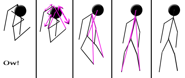
Next we can create the body. I added each body part to somewhat accurately match the mass and length proportions of a regular human body. Check out Body.pde in the source files for full details. Doing this will lead us to another issue: the body will easily contort into awkward shapes, and look very unrealistic.
There are a number of ways to fix this. In the demo, we use invisible and very unstiff links from the feet to the shoulder and the pelvis to the head in order to naturally push the body into a less awkward resting position.
You can also create fake-angle constraints by using links. Lets say we have three PointMasses, with two linked to one in the middle. You can find a length between the ends in order to satisfy any chosen angle. To find that length, you can use the Law of Cosines.
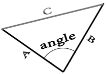
A = resting distance from end PointMass to center PointMass
B = resting distance from other PointMass to center PointMass

length = sqrt(A*A + B*B - 2*A*B*cos(angle))

create link between end PointMasses using length as resting distance
Modify the link so that this constraint will only apply when the distance is less than the resting distance, or, if it’s more than. This will keep the angle at the center point from ever being too close or too far, depending on what you need.
Step 9: More Dimensions!
One of the great things with having a completely linear physics engine is the fact that it can be any dimension you’d like. Everything done to x was also done to a y value, and thereforce can be exended to three or even four dimensions (I’m not sure how you’d render that, though!)
For example, here’s a link constraint for the simulation in 3D:
// calculate the distance
diffX = p1.x - p2.x
diffY = p1.y - p2.y
diffZ = p1.z - p2.z
d = sqrt(diffX * diffX + diffY * diffY + diffZ * diffZ)

// difference scalar
difference = (restingDistance - d) / d

// translation for each PointMass. They'll be pushed 1/2 the required distance to match their resting distances.
translateX = diffX * 0.5 * difference
translateY = diffY * 0.5 * difference
translateZ = diffZ * 0.5 * difference

p1.x += translateX
p1.y += translateY
p1.z += translateZ

p2.x -= translateX
p2.y -= translateY
p2.z -= translateZ
Conclusion
Thanks for reading! Much of the simulation is heavily based off of Thomas Jakobsen’s Advanced Character Physics article from GDC 2001. I did my best to strip most of the complicated stuff, and simplify to the point that most programmers will understand. If you need help, or have any comments, feel free to post below.